Arbitrage
Arbitrage is the trading of currencies for a profit. Arbitrage is a very real problem that promises a lot of money, if it were not for fees, taxes, and other imposed bounds. The challenge in arbitrage is finding an optimal solution despite the size of the search space. For example, for a set of 20 currencies, the search space consists of $@3 \times 10^{24}@$ (read “three septillion” in the short scale) different ways to trade currencies. In this article we explain how to solve the problem Arbitrage by UVa Online Judge.
Arbitrage is problem 104 in the UVa Online Judge. Even though I include the problem description in this post, I encourage you to visit the UVa Online Judge because there you will be able to submit your solution to get it judged.
Problem
Arbitrage is the trading of one currency for another with the hopes of taking advantage of small differences in conversion rates among several currencies in order to achieve a profit. For example, if 1.00 in U.S. currency buys 0.7 British pounds currency, 1.00 in British currency buys 9.5 French francs, and 1 French franc buys 0.16 in U.S. dollars, then an arbitrage trader can start with 1.00 USD and earn 1 * 0.7 * 9.5 * 0.16 = 1.064 dollars thus earning a profit of 6.4 percent.
You will write a program that determines whether a sequence of currency exchanges can yield a profit as described above.
To result in successful arbitrage, a sequence of exchanges must begin and end with the same currency, but any starting currency may be considered.
Input
The input file consists of one or more conversion tables. You must solve the arbitrage problem for each of the tables in the input file. Each table is preceded by an integer $@n@$ on a line by itself giving the dimensions of the table. The maximum dimension is 20. The minimum dimension is 2.
The table then follows in row major order but with the diagonal elements of the table missing (these are assumed to have value 1.0). Thus the first row of the table represents the conversion rates between country 1 and $@n - 1@$ other countries, i.e. the amount of currency of country $@i@$ constrained to $@2 \leq i \leq n@$ that can be purchased with one unit of the currency of country 1.
Thus each table consists of $@n + 1@$ lines in the input file: 1 line containing $@n@$ and $@n@$ lines representing the conversion table.
Output
For each table in the input file, you must determine whether a sequence of exchanges exists that results in a profit of more than 1 percent (0.01). If a sequence exists you must print the sequence of exchanges that results in a profit. If there is more than one sequence that results in a profit of more than 1 percent you must print a sequence of minimal length, i.e. one of the sequences that uses the fewest exchanges of currencies to yield a profit.
Because the IRS (United States Internal Revenue Service) taxes long
transaction sequences with a high rate, all profitable sequences must
consist of $@n@$ or fewer transactions where $@n@$ is the dimension of
the table giving conversion rates. The sequence 1 2 1 represents
two conversions.
If a profitable sequence exists you must print the sequence of exchanges that results in a profit. The sequence is printed as a sequence of integers with the integer $@i@$ representing the $@i@$-th line of the conversion table (country $@i@$). The first integer in the sequence is the country from which the profitable sequence starts. This integer also ends the sequence.
If no profiting sequence of $@n@$ or fewer transactions exists, then the line
no arbitrage sequence existsshould be printed.
Sample Input
3
1.2 .89
.88 5.1
1.1 0.15
4
3.1    0.0023    0.35
0.21   0.00353   8.13
200    180.559   10.339
2.11   0.089     0.06111
2
2.0
0.45
Sample Output
1 2 1
1 2 4 1
no arbitrage sequence exists
Analysis
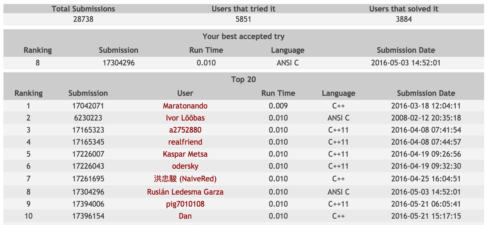
For a given problem, the conversion table corresponds to a graph and the solution corresponds to a shortest profitable cycle in that graph. Consider the following conversion table over USD, MXN, and EUR.
3
1.004987562112089 1.004987562112089
0.99503719020999 1.004987562112089
1.004987562112089 0.99503719020999
The table corresponds to the following interpretation.
     | USD         | MXN         | EUR
----------------------------------------------
 USD | 0           | 1.01^(1/2)  | 1.01^(1/2)
 MXN | 1.01^(-1/2) | 0           | 1.01^(1/2)
 EUR | 1.01^(1/2)  | 1.01^(-1/2) | 0
The corresponding graph is the following.
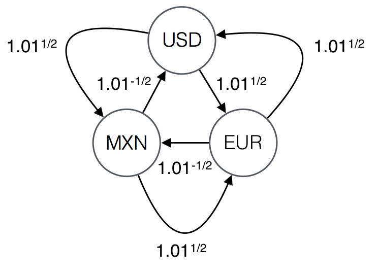
When we interpret the conversion table, we write 0 for the rates in the diagonal to indicate that we do not consider edges that start and end in the same vertex.
The reason is that those edges are redundant.
A lasso is an edge that starts and ends in the same vertex.
Lassos are redundant because from a given sequence that includes a lasso you obtain a shorter sequence with the same rate by removing the lasso.
For example, sequence USD USD EUR USD yields profit 1.01, the same profit that the shorter sequence USD EUR USD yields.
A sequence of exchanges may yield a profit only if the sequence is a cycle.
For example, the cycle USD -> MXN -> EUR -> USD yields profit of $@1.01^{3/2}@$.
Given that the number of vertices in the graph is 3, we do not consider cycles longer than 3.
Consider the cycles of length 3 or less.
CYCLE                    : RATE

USD -> MXN -> USD        : 1
USD -> EUR -> USD        : 1.01
EUR -> MXN -> EUR        : 1
USD -> MXN -> EUR -> USD : 1.01^(3/2)
USD -> EUR -> MXN -> USD : 1.01^(-1/2)
A cycle is profitable when its rate is greater or equal to 1.01. Out of the five cycles, only the following two are profitable.
USD -> EUR -> USD
USD -> MXN -> EUR -> USD
Out of the two profitable cycles, USD -> EUR -> USD is the only solution because it is the shortest cycle.
A solution may not be a simple cycle like in the previous example. For example, consider the following conversion table and its corresponding graph.
4
1 0 0
1.005 0 0
0 0 0
0 0 0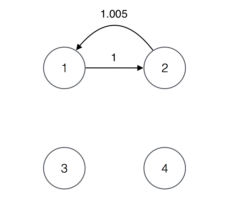
For the graph, the cycles of length 4 or less are the following
CYCLE     : RATE
1 2 1     : 1.005
1 2 1 2 1 : 1.010025
The only profitable cycle is 1 2 1 2 1 and therefore it is the only solution.
The cycle is a solution regardless of the fact that it consists of the repetition of simple cycle 1 2 1.
A solution that is not a simple cycle is not necessarily the repetition of a simple cycle like in the previous example. For example, consider the following conversion table and its corresponding graph.
5
1.001992047666533 0 0 1.001992047666533
1.001992047666533 0 0 0
1.001992047666533 0 0 0
0 0 0 0
0 0 1.001992047666533 0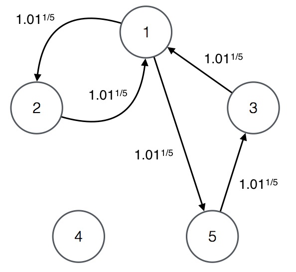
For the graph, the cycles of length 5 or less are the following.
CYCLE       : RATE
1 2 1       : 1.01^(2/5)
1 5 3 1     : 1.01^(3/5)
1 2 1 5 3 1 : 1.01
The only profitable cycle is 1 2 1 5 3 1 and therefore it is the only solution.
The cycle consists of simple cycles 1 2 1 and 1 5 3 1.
Searching for a solution is difficult because there may be many cycles for a given problem. The reason is that a conversion table of length $@n@$ corresponds to complete graph $@K_n@$. Even if there are edges with weight 0, we consider them because considering a complete graph makes for a simpler solution. The exception are lassos, which we do not consider because they are redundant. For complete graphs of size $@2 \leq n \leq 20@$, the number of cycles of length $@n@$ or less is the following.
 K2:                                       1
 K3:                                       5
 K4:                                      42
 K5:                                     384
 K6:                                   4,665
 K7:                                  69,537
 K8:                               1,230,124
 K9:                              25,140,552
K10:                             582,508,305
K11:                          15,084,077,381
K12:                         431,646,196,806
K13:                      13,525,545,361,080
K14:                     460,576,563,322,057
K15:                  16,935,036,272,292,001
K16:                 668,691,718,661,091,000
K17:              28,220,125,532,003,984,176
K18:           1,267,597,789,008,779,578,401
K19:          60,381,304,029,673,985,693,205
K20:       3,040,239,935,992,309,703,757,730
Approach
We approach the problem by searching for a shortest profitable cycle amongst a limited number of candidates.
We guarantee that the profitable cycle we find is shortest by considering candidates in order of length.
Consider the following input graph.
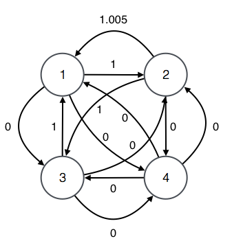
The candidates of length 2 are the cycles of length 2. Thus, we consider the cycles of length 2 from each one of the vertices as illustrated in the following diagram. These are all the cycles of length 2 because we consider all paths that start and end in each given vertex.
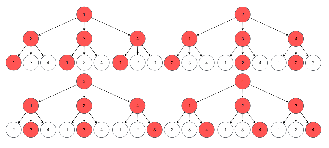
We search for a profitable candidate of length 2 by considering each root and each corresponding child.
For example, for root 1 and child 2, we consider the following candidate.
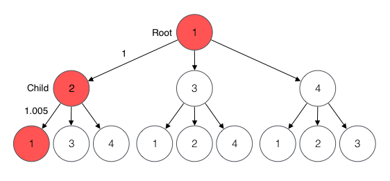
The rate of the candidate is 1.005 which is not profitable and therefore not a solution.
We search the rest of the candidates by repeating the process for each root and child.
We find no profitable candidate of length 2.
Half of the candidates of length 2 are repeated but we consider them anyway.
For example, candidate for root 2 and child 1 (2 -> 1 -> 2) is the same cycle and candidate for root 1 and child 2 (1 -> 2 -> 1).
The reason we consider repetitions is that when we apply the process to longer candidates, the number of candidates we consider for each length remains 12 while the number of cycles for the length increases.
For example, when we consider candidates of length 4 for the input graph, we consider 12 candidates instead of the 28 cycles of length 4 that exist.
Given that there is no solution of length 2, we search for a profitable candidate of length 3.
The candidates of length 3 are most beneficial cycles of length 3.
The structure of each candidate consists of a prefix edge i -> j and a suffix path j -> k -> i.
For example, the candidate for root 1 and child 2 is the following.
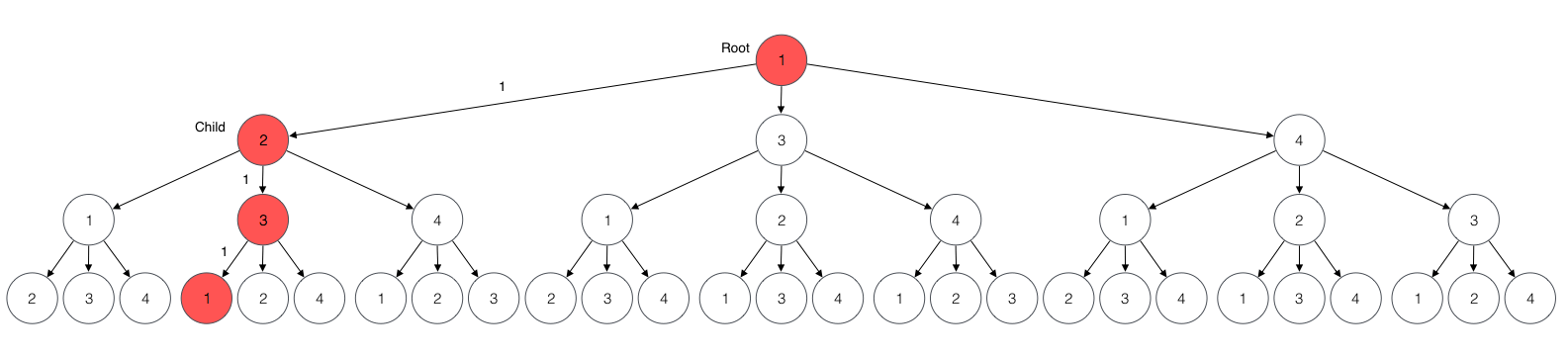
The prefix edge 1 -> 2 is the edge from 1 to 2 given by the input graph.
The suffix path 2 -> 3 -> 1 is a most beneficial path of length 2 from 2 to 1.
In this case the suffix is the most beneficial path of length 2 from 2 to 1.
The rate of the candidate is 1 which is not profitable and therefore not a solution.
Given that there is a candidate for each root and child, we search the rest of the candidates by repeating the process for each root and child.
We find no profitable candidate of length 3.
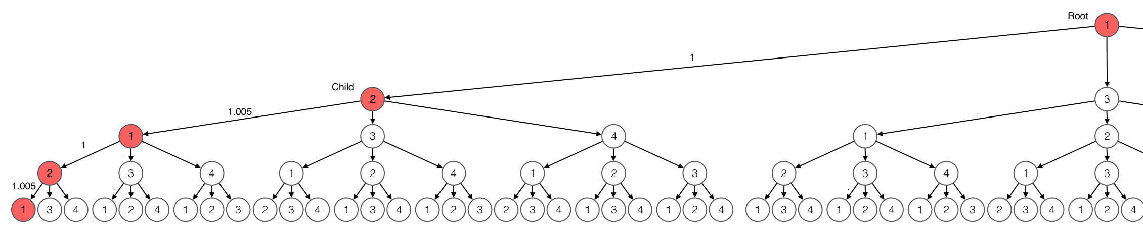
Candidates are most beneficial paths, for that reason we construct candidates by constructing most beneficial paths.
The construction of most beneficial paths is determined by their structure. Consider the structure a most beneficial path.
p = i -> k -> ... -> j
    ------------------
             |
          m edges
The candidate consists of a prefix edge i -> k and a suffix path k -> ... -> j.
The suffix path is a most beneficial path of length 2 from k to j because p is a most beneficial path.
If the suffix were not most beneficial, p would not be a most beneficial path from i to j because there would be a suffix from k to j with a higher rate.
The rate B'[i,j] of path p is determined by the rate of its edge W[i,k] and the rate of its suffix B[k,j] as follows.
B'[i,j] = W[i,k] * B[k,j]The construction of a most beneficial path corresponds to the calculation of its rate.
For given origin i and destination j vertices, we obtain the rate B[m][i,j] of most beneficial path of length m from the rates of most beneficial paths of length m - 1 as follows.
B[m][i,j] = max { W[i,k] * B[m - 1][k,j] | k in 1 ... n }For the matrix of weights W corresponding to the input graph, the rate of most beneficial paths of length 1 B[1] is W.
It is possible to construct most beneficial paths on demand instead of upfront together with candidates.
We do not explain that approach because the time complexity of the end-to-end algorithm is the same either way.
We do provide an implementation of the approach for reference.
When we construct most beneficial paths, we consider many more paths than the count of candidates. While we consider 12 candidates for each length, we consider 48 paths when we compute most beneficial paths (4 roots times 3 children times 4 destination vertices). We do so because for a given input graph, the number of candidates is constant for each length and thus the total count of paths that we consider is much less than the count of cycles in the graph. Compare the overapproximation $@n^4@$ of count of paths we consider to the number of cycles in the input graph.
                NUMBER OF CYCLES                   NUMBER OF PATHS WE CONSIDER
 K2:                                       1   <                16
 K3:                                       5   <                81
 K4:                                      42   <               256
 K5:                                     384   <               625
 K6:                                   4,665   >              1296
 K7:                                  69,537   >              2401
 K8:                               1,230,124   >              4096
 K9:                              25,140,552   >              6561
K10:                             582,508,305   >             10000
K11:                          15,084,077,381   >             14641
K12:                         431,646,196,806   >             20736
K13:                      13,525,545,361,080   >             28561
K14:                     460,576,563,322,057   >             38416
K15:                  16,935,036,272,292,001   >             50625
K16:                 668,691,718,661,091,000   >             65536
K17:              28,220,125,532,003,984,176   >             83521
K18:           1,267,597,789,008,779,578,401   >            104976
K19:          60,381,304,029,673,985,693,205   >            130321
K20:       3,040,239,935,992,309,703,757,730   >            160000
The overapproximation corresponds to our nested iteration of $@n@$ lengths, $@n@$ roots, $@n@$ children, and $@n@$ destination vertices.
Given that there is no solution of length 3, we search for a profitable candidate of length 4. For root 1 and child 2, the candidate is the following.
The prefix edge 1 -> 2 is given by the input graph.
The suffix path is the most beneficial path of length 3 from 2 to 1.
In this case there is only one most beneficial path, 2 1 2 1.
The rate of the candidate is 1.010025 which is profitable and thus a solution.
We stop and return the solution.
If we repeated the process for the other candidates, we would find no other solution.
Thus, 1 2 1 2 1 is the only solution.
Algorithm
We present algorithms S, S’, and R.
Our solution is algorithm S’.
Algorithm S is a summary of algorithm S’ and is easier to understand.
Algorithm R is an alternative to algorithm S that computes most beneficial paths on demand.
The execution time of the three algorithms is $@O(n^4)@$.
S(n, W)
 1: B[1] := W
 2: FOR m := 2 TO n
 3:     B[m] := 0
 4:     FOR i := 1 TO n
 5:         FOR j := 1 TO n
 6:             FOR k := 1 TO n
 7:                 IF B[m][i,j] < W[i,k] * B[m - 1][k,j]
 8:                     B[m][i,j] = W[i,k] * B[m - 1][k,j]
 9:                     IF B[m][i,i] >= 1.01
10:                         RETURN B[m][i,i]
11: RETURN 0
Algorithm S returns the rate of a solution or zero if there is no solution for given weight matrix W of size $@n \times n@$,
Algorithm S finds a solution rate by constructing rates of candidates of increasing length and returning the first rate that is profitable.
Algorithm S constructs rates of candidates by constructing rates of most beneficial paths.
The reason is that candidates are most beneficial paths.
The following is algorithm S’.
S'(n, W)
 1: B[1] := W
 2: FOR i := 1 TO n
 3:     FOR j := 1 TO n
 4:         IF W[i,j] > 0
 5:             P[1][i,j] := j
 6: FOR m := 2 TO n
 7:     B[m] := 0
 8:     FOR i := 1 TO n
 9:         FOR j := 1 TO n
10:             FOR k := 1 TO n
11:                 IF B[m][i,j] < W[i,k] * B[m - 1][k,j]
12:                     B[m][i,j] = W[i,k] & B[m - 1][k,j]
13:                     P[m][i,j] = k
14:                     IF B[m][i,i] >= 1.01
15:                         RETURN m, i, B, P
16: RETURN 0
Algorithm S’ returns a solution and its rate when there is one.
If there is no solution, algorithm S’ returns zero.
Algorithm S’ computes rates of most beneficial paths in the way algorithm S does and at the same time constructs a solution in successor matrix P.
Algorithm S’ constructs a solution by recording the successor k of vertex i in P[m][i,j] in line 13.
Algorithm S’ stops as soon as it finds a profitable candidate in line 14.
R(n, W)
 1: B[0] := Identity matrix n x n
 2: B[1] := 0
 3: FOR m := 2 TO n
 4:     B[m] := 0
 5:     FOR i := 1 TO n
 6:         FOR j := i + 1 TO n
 7:             FOR k := i TO n
 8:                 IF B[m - 1][j,i] < W[j,k] * B[m - 2][k,i]
 9:                     B[m - 1][j,i] = W[j,k] * B[m - 2][k,i]
12:             IF B[m][i,i] < W[i,j] * B[m - 1][j,i]
13:                 B[m][i,i] = W[i,j] * B[m - 1][j,i]
14:                 IF B[m][i,i] >= 1.01
15:                     RETURN B[m][i,i]
16: RETURN 0
Algorithm R computes the same result as algorithm S by constructing most beneficial paths on demand. We include algorithm R to illustrate that the time complexity of constructing most beneficial paths on demand is the same as the complexity of constructing them upfront. The reason is that algorithms S and R both run in time $@O(n^4)@$ because each has four nested loops.
Implementation
The following C program is our implementation of algorithm S’.
For a given weight matrix rate of size $@n \times n@$, function S executes algorithm S’ and prints a solution if there is one.
If there is no solution, function S prints “no arbitrage sequence exists.”
#include <stdio.h>

#define V 20
#define MIN_PROFIT 1.01

#define Si(n) scanf("%d", &n)
#define Sf(n) scanf("%f", &n)

void print_path(int s, int t, int l, int succ[V][V][V]) {
  if(l == 0)
    printf("%d\n", s + 1);
  else {
    printf("%d ", s + 1);
    print_path(succ[l][s][t], t, l - 1, succ);
  }
}

void set_to_zero(int n, float m[V][V]) {
  int i, j;
  for(i = 0; i < n; i++)
    for(j = 0; j < n; j++)
      m[i][j] = 0;
}

void S(int n, float rate[V][V]) {
  float benefit[V][V][V];
  int succ[V][V][V];
  int l, i, j, k;
  for(i = 0; i < n; i++)
    for(j = 0; j < n; j++) {
      benefit[1][i][j] = rate[i][j];
      if(rate[i][j] > 0)
        succ[1][i][j] = j;
    }
  for(l = 2; l <= n; l++) {
    set_to_zero(n, benefit[l]);
    for(i = 0; i < n; i++)
      for(j = 0; j < n; j++)
        for(k = 0; k < n; k++) {
          if(benefit[l][i][j] < rate[i][k] * benefit[l - 1][k][j]) {
            benefit[l][i][j] = rate[i][k] * benefit[l - 1][k][j];
            succ[l][i][j] = k;
            if(benefit[l][i][i] >= MIN_PROFIT) {
              print_path(i, i, l, succ);
              return;
            }
          }
        }
  }
  printf("no arbitrage sequence exists\n");
}

int main() {
  int n, i, j;
  float r;
  float rate[V][V];
  while(Si(n) != EOF) {
    for(i = 0; i < n; i++)
      for(j = 0; j < n; j++) {
        if(i == j) {
          rate[i][i] = 0;
          continue;
        }
        Sf(r);
        rate[i][j] = r;
      }
    S(n, rate);
  }
  return 0;
}
We present our C implementation of algorithm R for reference.
Our implementation computes the rate of the solution as well as the solution path.
The main difference is that this program separates the construction of candidates from the construction of most beneficial paths.
In function R, the construction of candidates happens in if block C and the construction of most beneficial paths happens in loop P.
#include <stdio.h>

#define V 20
#define MIN_PROFIT 1.01

#define Si(n) scanf("%d", &n)
#define Sf(n) scanf("%f", &n)

void print_path(int s, int t, int l, int succ[V+1][V][V]) {
  if(l == 0)
    printf("%d\n", s + 1);
  else {
    printf("%d ", s + 1);
    print_path(succ[l][s][t], t, l - 1, succ);
  }
}

void set_to_zero(int n, float m[V][V]) {
  int i, j;
  for(i = 0; i < n; i++)
    for(j = 0; j < n; j++)
      m[i][j] = 0;
}

void R(int n, float rate[V][V]) {
  float benefit[V+1][V][V];
  int succ[V+1][V][V];
  int l, i, j, k;
  set_to_zero(n, benefit[0]);
  for(i = 0; i < n; i++)
    benefit[0][i][i] = 1;
  set_to_zero(n, benefit[1]);
  for(l = 2; l <= n; l++) {
    set_to_zero(n, benefit[l]);
    for(i = 0; i < n; i++)
      for(j = i + 1; j < n; j++) {
        for(k = i; k < n; k++)  /* ....................................... P */
          if(benefit[l - 1][j][i] < rate[j][k] * benefit[l - 2][k][i]) {
            benefit[l - 1][j][i] = rate[j][k] * benefit[l - 2][k][i];
            succ[l - 1][j][i] = k;
          }
        if(benefit[l][i][i] < rate[i][j] * benefit[l - 1][j][i]) { /* .... C */
          benefit[l][i][i] = rate[i][j] * benefit[l - 1][j][i];
          succ[l][i][i] = j;
          if(benefit[l][i][i] >= MIN_PROFIT) {
            print_path(i, i, l, succ);
            return;
          }
        }
      }
  }
  printf("no arbitrage sequence exists\n");
}

int main() {
  int n, i, j;
  float r;
  float rate[V][V];
  while(Si(n) != EOF) {
    for(i = 0; i < n; i++)
      for(j = 0; j < n; j++) {
        if(i == j) {
          rate[i][i] = 0;
          continue;
        }
        Sf(r);
        rate[i][j] = r;
      }
    R(n, rate);
  }
  return 0;
}
The worst time complexity of function R is the same as that of function S, $@O(n^4)@$.
The UVa Online Judge reports the same execution time for both programs, 0.010 seconds.
We obtained 8th place by submitting function R.
The rank is still the same as of 2016.05.26.
Subsequent submission of function S produced the same execution time.
Related work
Algorithmist, OurQuestToSolve, and Chang suggest that this problem can be solved by modifying Floyd-Warshall.
Algorithm S is the algorithm described by those sites.
We agree with Prajogo Tio in that Algorithm S only resembles Floyd-Warshall.
We explain that a more similar algorithm is Slow All Pairs Shortest Paths by Cormen et al.
Consider Floyd-Warshall.
FloydWarshall(n, W)
1: D[0] = W
2: FOR k := 1 TO n
3:     FOR i := 1 TO n
4:         FOR j := 1 TO n
5:             IF D[k - 1][i,j] > D[k - 1][i,k] + D[k - 1][k,j]
6:                 D[k][i,j] = D[k - 1][i,j]
7:             ELSE
8:                 D[k][i,j] = D[k - 1][i,k] + D[k - 1][k,j]
9: RETURN D[n]
Cormen et al explain how Floyd-Warshall constructs shortest paths for all pairs of vertices for a graph given by adjacency matrix W of size $@n \times n@$.
Algorithm S is not similar to Floyd-Warshall because Floyd-Warshall considers intermediate vertices in each iteration of its outer loop instead of an increasing number of edges.
Floyd-Warshall considers that the structure of a shortest path consists of a shortest prefix, an intermediate vertex, and a shortest suffix.
                    suffix
                      |
                -------------
p = i -> ... -> k -> ... -> j
    -------------\
          |       \
       prefix      \
               intermediate
                  vertex
The intermediate vertex k is neither the origin vertex of p nor the destination vertex.
Floyd-Warshall refines shortest paths with each iteration of its outer loop by considering the paths corresponding to each intermediate vertex.
In the first iteration, the shortest distance D[0][i,j] from i to j is the value given by given adjacency matrix W.
D[0][i,j] = W[i,j]The assignment is implemented in line 1.
In iteration k, Floyd-Warshall considers the paths that visit vertex k as intermediate vertex and applies the refinement rule FW-REF.
D[k][i,j] = min { D[k - 1][i,j], D[k - 1][i,k] + D[k - 1][k,j] } (FW-REF)The refinement rule indicates that the shortest distance D[k][i,j] from i to j is either the previous shortest distance or the distance of the shortest path that goes from i to j through k.
The refinement is implemented in lines 5 to 8.
After iteration k, shortest path D[k][i,j] consists of at most k edges.
Considering intermediate vertices like Floyd-Warshall is not an effective approach to solving Arbitrage. Consider the following graph.
The solution is 1 -> 3 -> 1.
The application of the Floyd-Warshall approach is the following.
We start with no intermediate vertices and thus the most beneficial paths are the edges of the graph.
We consider vertex 2.
 ORIG | DEST | PREV PATH | PREV RATE | REFINED PATH | REFINED RATE
-------------------------------------------------------------------
  1   |  1   | N/A       | N/A       | N/A          | N/A
  1   |  3   | 1 -> 3    | 1.01^1/2  | 1 -> 2 -> 3  | 1.01
  3   |  1   | 3 -> 1    | 1.01^1/2  | 3 -> 1       | 1.01^1/2
  3   |  3   | N/A       | N/A       | N/A          | N/A
We refine the most beneficial path from 1 to 3 because going through 2 is more beneficial than the edge 1 -> 3.
We do not refine the path from from 3 to 1 because going through 2 is not more beneficial than the edge 3 -> 1.
There is no path from 1 to 1 or 3 to 3 because we have not considered enough intermediate vertices.
Paths that begin or end in 2 remain the same because 2 is not an intermediate vertex.
We consider vertex 3.
 ORIG | DEST | PREV PATH | PREV RATE | REFINED PATH     | REFINED RATE
-------------------------------------------------------------------
  1   |  1   | N/A       | N/A       | 1 -> 2 -> 3 -> 1 | 1.01^3/2
  1   |  2   | 1 -> 2    | 1.01^1/2  | 1 -> 2           | 1.01^1/2
  2   |  1   | 2 -> 1    | 1.01^-1/2 | 2 -> 3 -> 1      | 1.01
  2   |  2   | N/A       | N/A       | N/A              | N/A
The refined path from 1 to 1 consists of prefix 1 -> 2 -> 3 and suffix 3 -> 1 because we apply refinement rule FW-REF.
That path is profitable so we return it as a solution.
But 1 -> 2 -> 3 -> 1 is not a solution because the only solution is 1 -> 3 -> 1.
Algorithm S does consider an intermediate node k, but it always constructs a most profitable path of a particular length.
The reason is that in every iteration of the outer loop, a most profitable path is constructed by prepending one more edge to a previous most profitable path.
Consider All Pairs Shortest Paths.
SlowAllPairsShortestPath(n, W)
1: D[0] = Identity matrix n x n
2: FOR m := 1 TO n
3:     D[m] := INFINITY
4:     FOR i := 1 TO n
5:         FOR j := 1 TO n
6:             FOR k := 1 TO n
7:                 IF D[m][i,j] > D[m - 1][i,k] + W[k,j]
8:                     D[m][i,j] = D[m - 1][i,j] + W[k,j]
9: RETURN D[n]
Cormen et al explain that All Pairs Shortest Paths constructs shortest paths that consist of at most m edges.
Algorithm S is similar to All Pairs Shortest Paths because both consider an increasing number of edges in each iteration of its outer loop.
All Pairs Shortest Paths considers that the structure of a shortest path consists of a shortest prefix and a suffix edge.
             suffix edge
                  |
                ------
p = i -> ... -> k -> j
    -------------
          |
       prefix path
  that is a shortest path
All Pairs Shortest Paths refines shortest paths with each iteration of its outer loop by extending current shortest path i -> ... -> k with one more edge k -> j.
The algorithm starts with the identity matrix in line 1.
The algorithm applies the following refinement rule.
D[m][i,j] = min( { D[m-1][i,j] } U { D[m-1][i,k] + W[k,j] | k in 1..n } )The refinement rule indicates that the shortest distance D[m][i,j] from i to j is either the previous shortest distance or the distance of extending some shortest path with and edge.
Algorithm S prepends one more edge to each most beneficial path in every iteration of its outer loop.
This is similar to the way Slow All Pairs Shortest Paths refines shortest paths.
There is a problem called Arbitrage by Sedgewick and Wayne that is similar to UVa’s Arbitrage problem.
Both ask for a sequence of exchanges that is profitable (i.e. with rate greater than 1).
The difference is that Sedgewick and Wayne ask for any simple cycle that is profitable and UVa asks for a cycle that is profitable by 1% and consists of the least amount of edges possible.
Because of the difference, Sedgewick and Wayne’s problem corresponds to finding a negative cycle and UVa’s problem does not.
We include work related to algorithm R for reference. Consider the following algorithm for enumerating simple cycles by Tarjan.
global vertex r
global stack path
global stack mark
global map mark_map

TarjanSimpleCycles(n, E)
 1: path := empty
 2: mark := empty
 3: FOR v := 1 TO n
 4:     mark_map[v] := FALSE
 5: FOR r := 1 TO n
 6:     Backtrack(r, n, E)
 7:     WHILE mark is not empty
 8:         v := POP(mark)
 9:         mark_map[v] := FALSE

Backtrack(v, n, E)
 1: found_cycle := FALSE
 2: PUSH(path, v)
 3: PUSH(mark, v)
 4: mark_map[v] := TRUE
 5: FOR w := r TO n
 6:     IF (v, w) not in E
 7:         CONTINUE
 8:     IF w = v
 9:         found_cycle := TRUE
10:         PRINT_PATH(path)
11:     ELSE IF not mark_map[w]
12:         found_cycle := found_cycle || Backtrack(r, w, n, E)
13: IF found_cycle
14:    WHILE PEEK(mark) != w
15:        w := pop(mark)
16:        mark_map[w] := FALSE
17:    POP(mark)
18:    mark_map[v] := FALSE
19: POP(path)
20: RETURN found_cycle
The way algorithm R considers paths is similar to the way of Tarjan’s algorithm enumerates simple cycles.
Algorithm R avoids repeated candidates by iterating all children j greater than root i in line 6 of R.
Algorithm R avoids considering most beneficial paths that have been considered in previous candidates by iterating all intermediate nodes k greater or equal than root i in line 7 of R.
The candidates and paths that algorithm R avoids correspond to the paths that Tarjan avoids by considering paths to all destinations w greater or equal than root r in line 5 of Backtrack.
Algorithm R considers non-simple cycles and Tarjan does not. For that reason the cycles that Tarjan avoids by means of mark_map in line 11 are considered by algorithm R.
Summary
Arbitrage is problem 104 in the UVa Online Judge. Arbitrage is a graph problem that asks for a cycle of minimum weight that is shortest. The challenge is that the number of cycles for a given input graph is exponential on the number of vertices. We approach the challenge by considering a limited set of candidates in increasing order of length. Our approach overcomes the challenge because we consider $@n^4@$ paths in the worst case, which is a much lower amount of paths than the number of cycles for more than half of the input sizes. Our approach corresponds to a popular solution found on the Internet that is usually considered similar to Floyd-Warshall when in reality only resembles Floyd-Warshall. Our approach is more similar to Slow All Pairs Shortest Paths by Cormen et al. The corresponding implementation is ranked 8th place as of 2016.05.26.
References
- [Algorithmist]
- "UVa 104." Algorithmist. N.p., 28 Jan. 2013. Web. 26 May 2016. http://www.algorithmist.com/index.php/UVa_104.
- [Chang]
- "[ACM] Some hints about uva 104 (Modified Floyd-Warshall)." 調和的靈感. N.p., 12 Jan. 2008. Web. 26 May 2016. http://chchwy.blogspot.mx/2008/12/acm-some-hint-about-uva-104.html.
- [Cormen et al]
- Cormen, Thomas H.; Leiserson, Charles E.; Rivest, Ronald L.; Stein, Clifford (2009) [1990]. In684-699n to Algorithms (3rd ed.). MIT Press and McGraw-Hill. pp. 1002-1012. ISBN 0-262-03384-4.
- [Prajogo Tio]
- "a bit of uva: UVa 104 - Arbitrage." A Bit of Cs. N.p., 8 Aug. 2014. Web. 26 May 2016. http://abitofcs.blogspot.mx/2014/08/a-bit-of-uva-uva-104-arbitrage.html.
- [OurQuestToSolve]
- "#104 - Arbitrage." Our Quest to Solve Them All. N.p. 2008. Web. 26 May 2016. http://www.questtosolve.com/browse.php?pid=104.
- [Sedgewick and Wayne]
- Sedgewick, Robert; Wayne, Kevin (2011). Algorithms (4th ed.). Addison-Wesley Professional. pp. 679-681. ISBN 978-0-321-57351-3.
- [Tarjan]
- Enumeration of the elementary circuits of a directed graph. R. Tarjan, SIAM Journal on Computing, 2(3) (1973), pp. 211-216