The Game of Life is a popular celular automaton that simulates the births and deaths of a population over time. Your task is to code an efficient implementation of the transition function. The rules of the game are the following.

The game models the population by means of a grid. Although the original game considers the infinite grid, we consider a finite grid so that anything outside the corresponding bounds is ignored. Consider the following example.

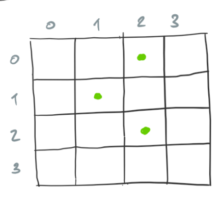
The cells marked with a dot are alive and the cells that are empty are dead.

Every cell, alive or dead, has up to 8 alive neighbors. The following diagram shows the neighbor cells of the cell marked with the green dot.

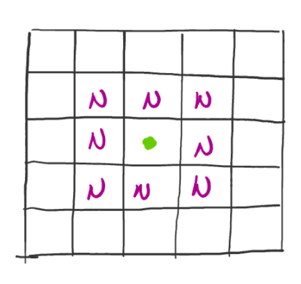
Time pases in discrete steps and each step corresponds to a configuration of the grid. The rules that govern the transition from one configuration to another are the following.

When a cell is alive and
1. it has less than 2 neighbors, it dies.
2. it has more than 3 neighbors, it dies.
3. it has 2 or 3 neighbors, it remains the alive.
When a cell is dead and
1. it has 3 neighbors, it becomes alive.
2. it has more or less than 3 neighbors, it remains dead.

For example, the following configuration is the successor of our previous example grid.

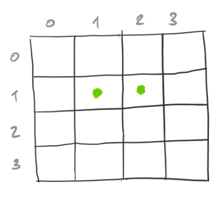
Because we find configurations that are have few alive cells more interesting, anything that you can do to improve performance for very large grids is welcome.

Input. The input consists of the size of the grid, followed by an initial configuration, followed by a number indicating the amount of steps to take from the initial step. The size of the grid is given on a single line as a pair of numbers, the The initial configuration begins with a number n on a separate line, the amount of cells that are alive. The rest of the initial configuration consits of n pairs of numbers, each on a separate line. The first number of each pair indicates the row and the second the column of a cell that is alive. The last line of the input is the amount of steps s to take from the initial configuration.

Output. The output consists of a sequence of pairs of row and column that corresponds to the cells that are alive after s steps. Each pair appears on a separate line.

1 1
1 2

Naive solution

A naive approach consists in counting the neighbors of each cell in the grid and then applying the rules to each cell. Consider the following configuration.

The count neighbors that correspond to each cell of the current configuration are the following.

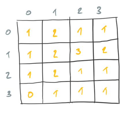
When we consider each count of neighbors, we find that only the following two cells are alive in the next configuration.

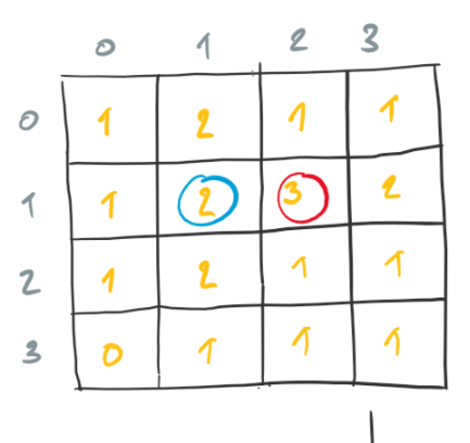
The following is the configuration we obtain by considering each count of neighbors.

The following is a Ruby implementation of our naive approach.

#!/usr/bin/env ruby

def populated_cells row, cols
  count = 0
  cols.each { |j|
    next if j < 0 || row.length <= j
    count += 1 if row[j]
  }
  return count
end

def neighbors curr, i, j
  count = 0
  if 0 < i
    count += populated_cells curr[i-1], [j-1, j, j+1]
  end
  count += populated_cells curr[i], [j-1, j+1]
  if i < curr.length - 1
    count += populated_cells curr[i+1], [j-1, j, j+1]
  end
  return count
end

def step curr
  succ = curr.map { |row| row.map { |_| false } }
  curr.each_with_index { |row, i|
    row.each_with_index { |cell, j|
      count = neighbors curr, i, j
      if count == 3 || cell && count == 2
        succ[i][j] = true
      end
    }
  }
  return succ
end

def main
  rows, cols = readline.split(' ').map(&:to_i)
  curr = (1..rows).map { |_| (1..cols).map { |_| false } }
  n = readline.to_i
  (1..n).each { |_|
    r, c = readline.split(' ').map(&:to_i)
    curr[r][c] = true
  }
  s = readline.to_i
  (1..s).each { |_| curr = step curr }
  curr.each_with_index { |row, i| row.each_with_index { |cell, j| puts "#{i} #{j}" if cell } }
end

main

The main function takes care of reading the initial configuration and number of steps. Function step implements the transition function for the automaton. Function step considers the count of neighbors and the state for each cell and acts accordingly. Function neighbors counts the neighbors for a given cell. Function neighbors uses function populated_cells to count alive cells out of the indicated cells in the given row.

The time and space complexity of this approach is O( rows * cols ).

Efficient solution

A more efficient approach is to only consider the neighbors of cells that are alive to determine the cells that are alive in the next configuration. Consider the following configuration.

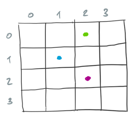
For each alive cell, we increase the count of neighbors for the corresponding neighbors. The following diagram shows the count of neighbors for neighbors of the cells that are alive.

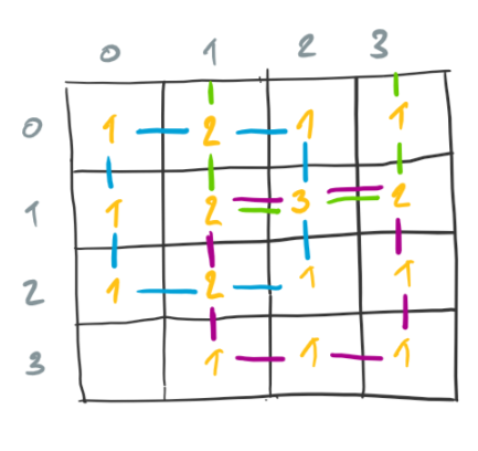
In the diagram, the neighbors corresponding to each alive cell are marked with lines of the same color as the alive cell.

Given the counts of neighbors, we consider each and the corresponding cell in the current configuration to determine if the cell should be alive in the successor configuration. The circled counts in the next diagram correspond to alive cells in the successor configuration. Note that it is unnecessary to consider the cell in the bottom-left corner, something we would have done in the naive approach.

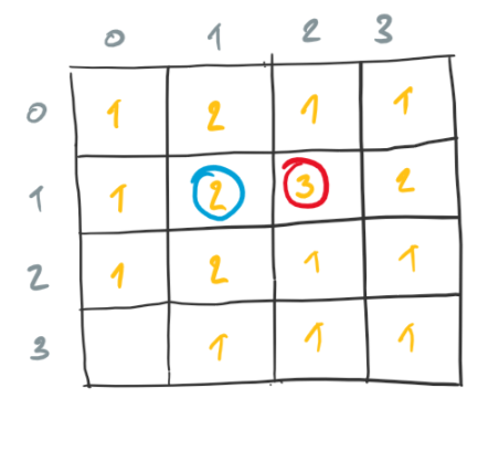
The following is a Ruby implementation of our efficient approach.

#!/usr/bin/env ruby

def increase_cells row, cells, cols
  cells.each { |c|
    next if c < 0 || c >= cols
    row[c] ||= 0
    row[c] += 1
  }
end

def step curr, rows, cols
  neighbors = {}
  curr.each { |r, row|
    row.each { |c, _|
      if r - 1 >= 0
        increase_cells (neighbors[r - 1] ||= {}), [c - 1, c, c + 1], cols
      end
      if r + 1 < rows
        increase_cells (neighbors[r + 1] ||= {}), [c - 1, c, c + 1], cols
      end
      increase_cells (neighbors[r] ||= {}), [c - 1, c + 1], cols
    }
  }
  succ = {}
  neighbors.each { |r, row|
    row.each { |c, count|
      if count == 3 || !!curr[r] && !!curr[r][c] && count == 2
        succ[r] ||= {}
        succ[r][c] = true
      end
    }
  }
  return succ
end

def main
  rows, cols = readline.split(' ').map(&:to_i)
  curr = {}
  n = readline.to_i
  (1..n).each { |_|
    r, c = readline.split(' ').map(&:to_i)
    curr[r] ||= {}
    curr[r][c] = true
  }
  s = readline.to_i
  (1..s).each { |_| curr = step curr, rows, cols }
  curr.each { |i, row| row.each { |j, cell| puts "#{i} #{j}" if cell } }
end

main

Function step computes the counts of neighbors using function increase_cells. Function increase_cells increases the cells on the given row as long as they are within bounds.

The time and space complexity of this approach is O( alive cells ).

Naive solution

Efficient solution

Comments